How to Calculate Microwave Fade Margin Accurately

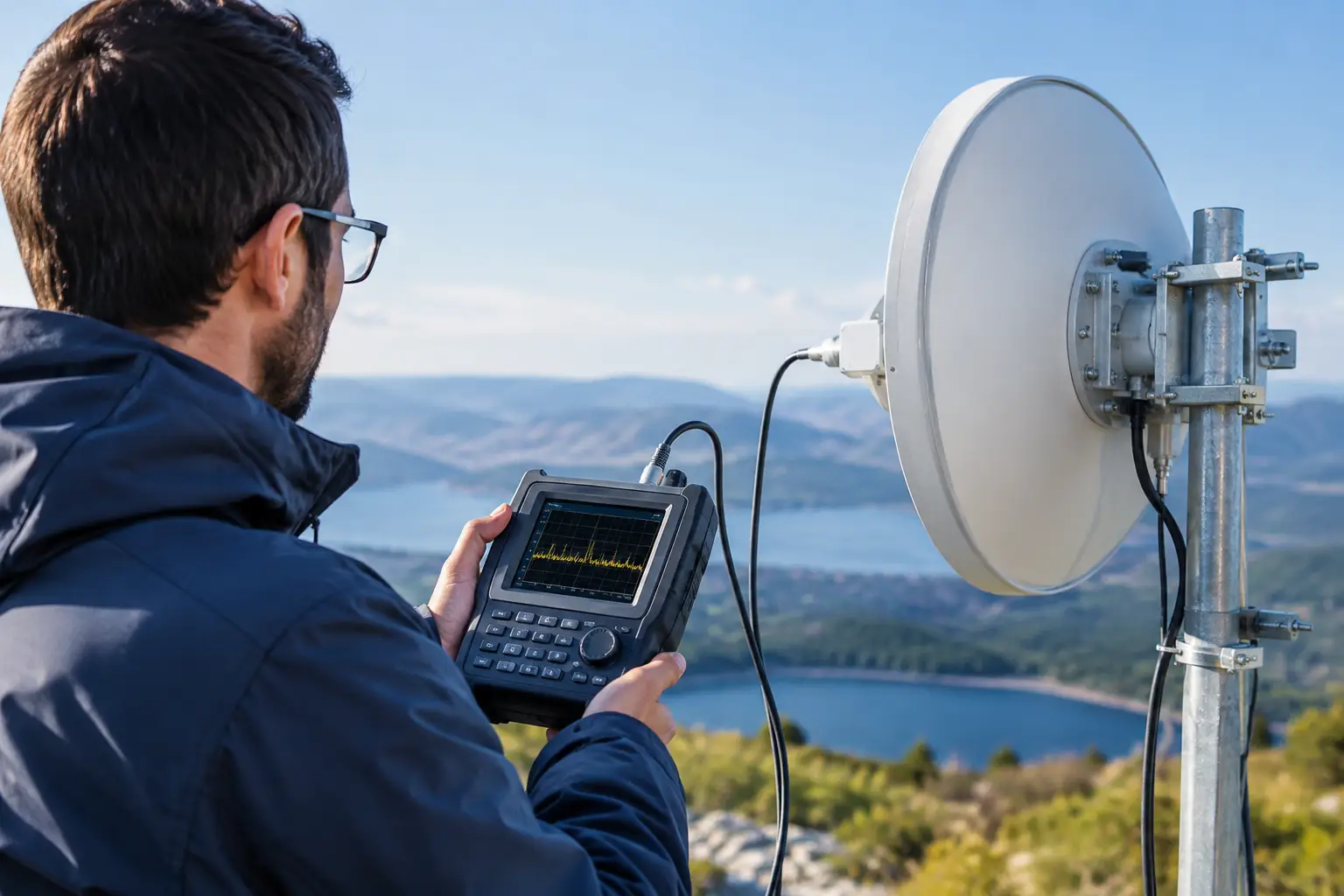
A microwave path can look excellent during commissioning and still fail its operational requirement months later, during a heavy rain cell, a temperature inversion, or a vessel roll event. To calculate microwave fade margin correctly, start with the received signal level under clear-air conditions, then measure that level against the receiver threshold required for the service you intend to deliver. The difference is the margin available to absorb real-world loss.

For mission-critical backhaul, that calculation is not a paperwork exercise. It determines whether a public safety command vehicle stays connected, whether an offshore platform retains operational communications, and whether a private LTE or 5G network has usable backhaul when conditions become difficult.

What Microwave Fade Margin Measures

Fade margin is the amount by which the received signal level (RSL) exceeds the receiver sensitivity threshold for a defined modulation, coding rate, channel bandwidth, and target error performance.

The basic calculation is:

Fade Margin (dB) = Received Signal Level (dBm) – Receiver Threshold (dBm)

If a receiver sees -58 dBm and its threshold for the selected mode is -72 dBm, the link has 14 dB of fade margin. In practical terms, the path can lose another 14 dB before the radio reaches that threshold.

That threshold must match the service objective. A radio may continue passing traffic at a lower modulation rate after it can no longer support its peak capacity. Therefore, a link might have 25 dB of margin for a reduced-rate modulation mode but only 10 dB for its committed throughput. For networks carrying surveillance video, control traffic, voice, or private cellular backhaul, those are materially different availability outcomes.

How to Calculate Microwave Fade Margin From a Link Budget

A dependable calculation begins with a complete link budget, not a free-space path loss figure alone. The clear-air RSL can be expressed as:

RSL = Transmit Power – Transmit Losses + Transmit Antenna Gain – Path Loss – Other Propagation Losses + Receive Antenna Gain – Receive Losses

All values are in dB or dBm. The components generally include transmit power, feeder or waveguide losses, antenna gains, free-space path loss, atmospheric absorption, radome loss, polarization losses, connector losses, and receive-side losses.

Free-space path loss is commonly calculated as:

FSPL (dB) = 92.45 + 20 log10(Frequency in GHz) + 20 log10(Distance in km)

Consider a 6 GHz, 30 km point-to-point path. Its free-space loss is approximately 137.6 dB. If the radio delivers 23 dBm, each antenna provides 34 dBi gain, and combined non-propagation losses total 3 dB, the estimated RSL is:

23 + 34 + 34 – 137.6 – 3 = -49.6 dBm

If the receiver threshold is -72 dBm at the planned modulation and coding rate, the preliminary fade margin is 22.4 dB. That is a useful starting result, but it is not yet a validated availability design. The remaining work is determining whether 22.4 dB covers the fading mechanisms at that site and frequency.

Use the Correct Receiver Threshold

Receiver sensitivity data is often misunderstood. Manufacturers may publish thresholds for several channel widths, modulation levels, coding schemes, and error-rate criteria. Do not select the most favorable number in the table unless that mode represents the capacity and quality of service the network must sustain.

Also account for receiver degradation caused by co-channel interference, adjacent-channel interference, and implementation conditions. A clean laboratory threshold is not always the right operational threshold on a congested tower, marine platform, or active field site. Where interference is credible, include an interference allowance or use a carrier-to-interference analysis alongside the thermal-noise calculation.

Include Losses That Drawings Often Miss

A link budget can be overstated by several dB when installation details are treated as minor. Radomes, flexible jumpers, waveguide runs, lightning protectors, adapters, and aging connectors all affect available margin. For stabilized and tracking systems, account for pointing error as well.

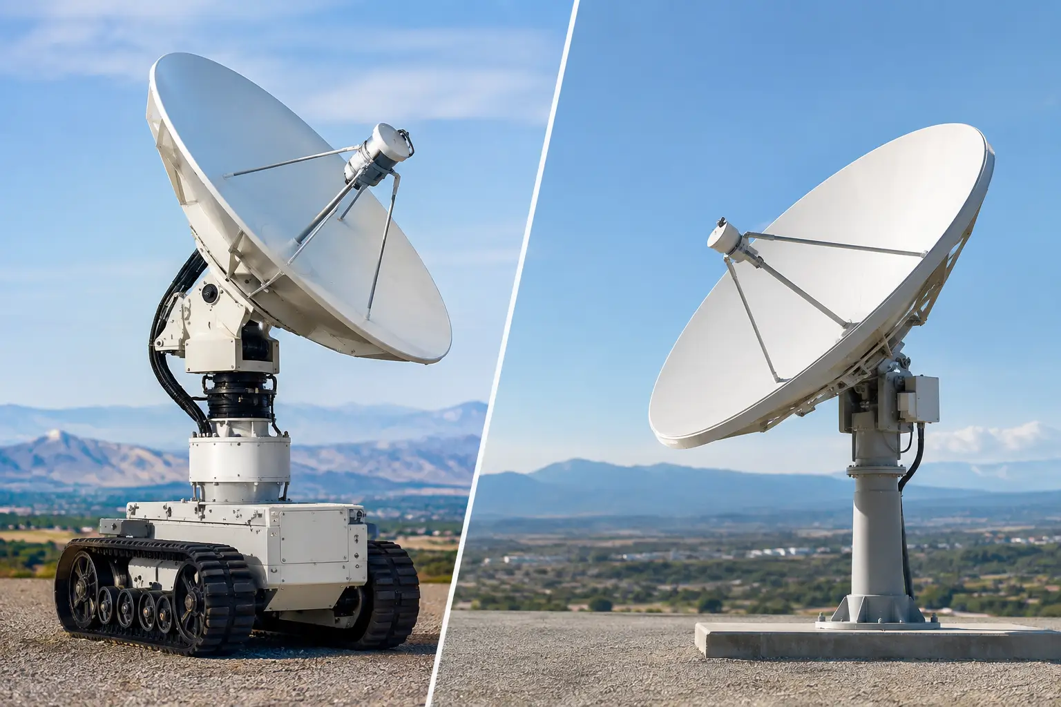
At narrow beamwidths, a small alignment offset can have a meaningful gain penalty. A fixed tower path and a ship-to-shore path should not receive the same pointing allowance. Mobile platforms introduce roll, pitch, yaw, vibration, changing geometry, and temporary obstruction. Auto-aiming antennas and stabilized microwave systems reduce these losses, but they do not remove the need to model the residual tracking and pointing error budget.

Match Fade Margin to the Dominant Fade Mechanism

The required margin depends on frequency, path length, climate, terrain, antenna heights, and availability target. A single rule such as “design for 20 dB” is not sufficient for engineered microwave networks.

Rain Fade at Higher Frequencies

Rain attenuation becomes a primary constraint as frequency increases, especially for long paths in the 11 GHz to 80 GHz range. A path that has substantial clear-air margin may lose that margin quickly during intense rainfall. Rain loss is frequency-dependent and must be estimated using local rainfall-rate data, path length, polarization, and the required annual availability.

For example, a short 18 GHz urban backhaul path may be practical with appropriate rain margin, while a longer path at the same frequency may require larger antennas, lower modulation, a shorter hop, or a different band. Higher-frequency spectrum can provide major capacity advantages, but it trades propagation tolerance for bandwidth.

Multipath and Atmospheric Fading

Below roughly 10 GHz, multipath fading can be more significant than rain. It occurs when reflected or refracted signal components arrive out of phase with the direct path. Paths over water, flat terrain, coastal corridors, and desert environments can be particularly susceptible, especially during atmospheric ducting conditions.

Multipath design is not solved solely by increasing transmit power. Antenna diversity, space diversity, frequency diversity, adaptive modulation, and carefully selected antenna heights may offer a better result. In some cases, changing tower elevation by a relatively small amount can improve the path profile and reduce the probability of severe fading.

Obstruction and Fresnel Zone Clearance

Fade margin cannot compensate for a path that is partially obstructed. The first Fresnel zone should be adequately clear along the route, with attention to terrain, vegetation growth, construction equipment, tidal conditions, and moving assets.

Partial Fresnel blockage adds variable diffraction loss and can create unstable performance that is difficult to diagnose from a static path survey. For industrial sites, plan for the operating environment rather than the empty-site condition. Cranes, stacks, vehicles, loading equipment, and seasonal foliage can all change the path.

Set an Availability Target Before Selecting Margin

The right fade margin follows the availability requirement. A best-effort construction-site link does not need the same design standard as a dispatch network, emergency response communications system, or offshore operational backhaul.

Availability is commonly expressed as a percentage over a year. A 99.9% target permits about 8.76 hours of annual downtime. At 99.99%, that falls to about 52.6 minutes. At 99.999%, the annual allowance is only about 5.3 minutes. The final increment looks small, but reaching it can change the antenna size, frequency plan, diversity architecture, and capital cost substantially.

This is where trade-offs should be made explicitly. More fade margin can come from higher-gain antennas, lower-loss RF components, shorter hops, lower-frequency spectrum, or reduced modulation. Each choice affects capacity, wind loading, licensing, cost, installation complexity, or network topology. For high-value traffic, a second path or diverse backhaul route may be more cost-effective than trying to force extreme availability from one radio hop.

Validate the Calculation in the Field

A modeled fade margin is only as reliable as its inputs. Confirm antenna alignment, actual transmit power, cable and waveguide loss, polarization, RSL, modulation behavior, and error statistics during commissioning. Record the baseline values so future degradation can be identified before a link fails.

For mobile and maritime deployments, validation must include movement. Test tracking acquisition, reacquisition after blockage, stabilization performance, and link behavior through expected vessel headings or vehicle operating conditions. The path is not static, so the acceptance test should not be static either.

BATS Wireless applies this engineering approach across fixed, mobile, maritime, and remote infrastructure deployments, combining path calculation with antenna tracking, stabilized microwave systems, and integrated radio compatibility. The objective is not merely to achieve a link at installation. It is to maintain the required service level under the conditions the operation will actually face.

The most useful fade-margin calculation is one that supports a decision: whether to change frequency, enlarge antennas, add diversity, adjust the path, or define a realistic throughput fallback. Build the margin around the service that must remain available when the environment stops cooperating.