What Is Link Budget? A Practical RF Design Guide

A microwave link can look excellent on a bench test and still fail at sea, on a moving vehicle, or across a remote industrial site. The difference is often understood before installation through one calculation: what is link budget? It is the accounting method that determines whether enough signal will arrive at a receiver, with sufficient margin, to support the required service under real operating conditions.

For organizations deploying long-range Wi-Fi, private LTE/5G, microwave backhaul, ground-to-air links, or onboard connectivity, link budget is not an academic RF exercise. It is a design control. It informs antenna selection, radio output, path length, mounting height, modulation choices, stabilization requirements, and the practical limits of a proposed network architecture.

What Is Link Budget in Wireless Engineering?

A link budget is a gain-and-loss calculation expressed in decibels (dB). It estimates the received signal level by starting with transmitted power, adding every gain in the path, and subtracting every loss between the transmitter and receiver.

At a basic level:

Received power = Transmit power + antenna gains – cable losses – path loss – environmental losses

The calculated received power is then compared with the receiver sensitivity required for the selected data rate, channel bandwidth, and modulation scheme. The difference between received power and receiver sensitivity is the available link margin.

A positive margin does not automatically mean a link is operationally acceptable. A static calculation may show a connection at a fixed location in clear weather, yet leave too little headroom for rain, vessel motion, vibration, interference, antenna misalignment, foliage growth, or equipment aging. Mission-critical designs require margin that reflects the conditions the system will actually face.

The Main Components of a Link Budget

Every RF system has a different architecture, but the same physical factors appear repeatedly. Good design begins by documenting them clearly rather than relying on nominal radio range claims.

Transmit Power and EIRP

Transmit power is the RF energy produced at the radio output, typically measured in dBm. A higher output can improve the budget, but it is only one variable. Regulatory EIRP limits, power consumption, heat, spectrum rules, and interference risk may restrict how much transmit power is practical or legal.

EIRP, or effective isotropic radiated power, combines radio transmit power with transmit antenna gain, minus losses between the radio and antenna. It is often the more useful number for evaluating the strength of the transmitted signal in the intended direction.

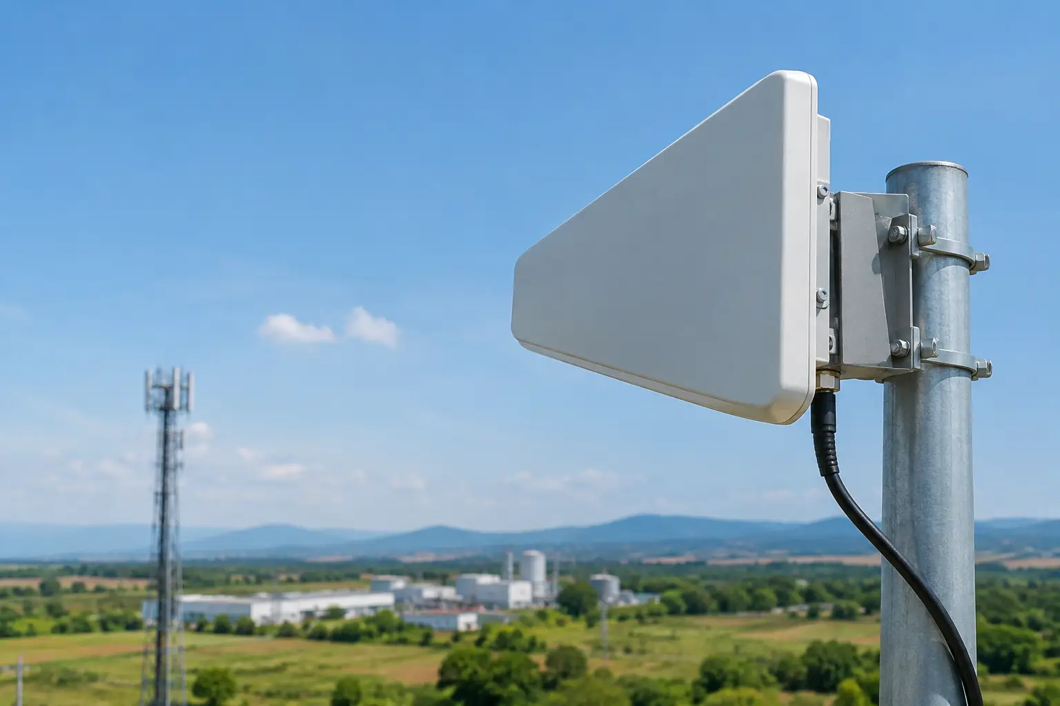
For example, a directional antenna can add substantial gain without increasing radio output power. That makes directional systems valuable for point-to-point backhaul, shore-to-vessel communications, and remote site connectivity. The trade-off is a narrower beamwidth, which increases the importance of accurate aiming and mechanical stability.

Antenna Gain and Polarization

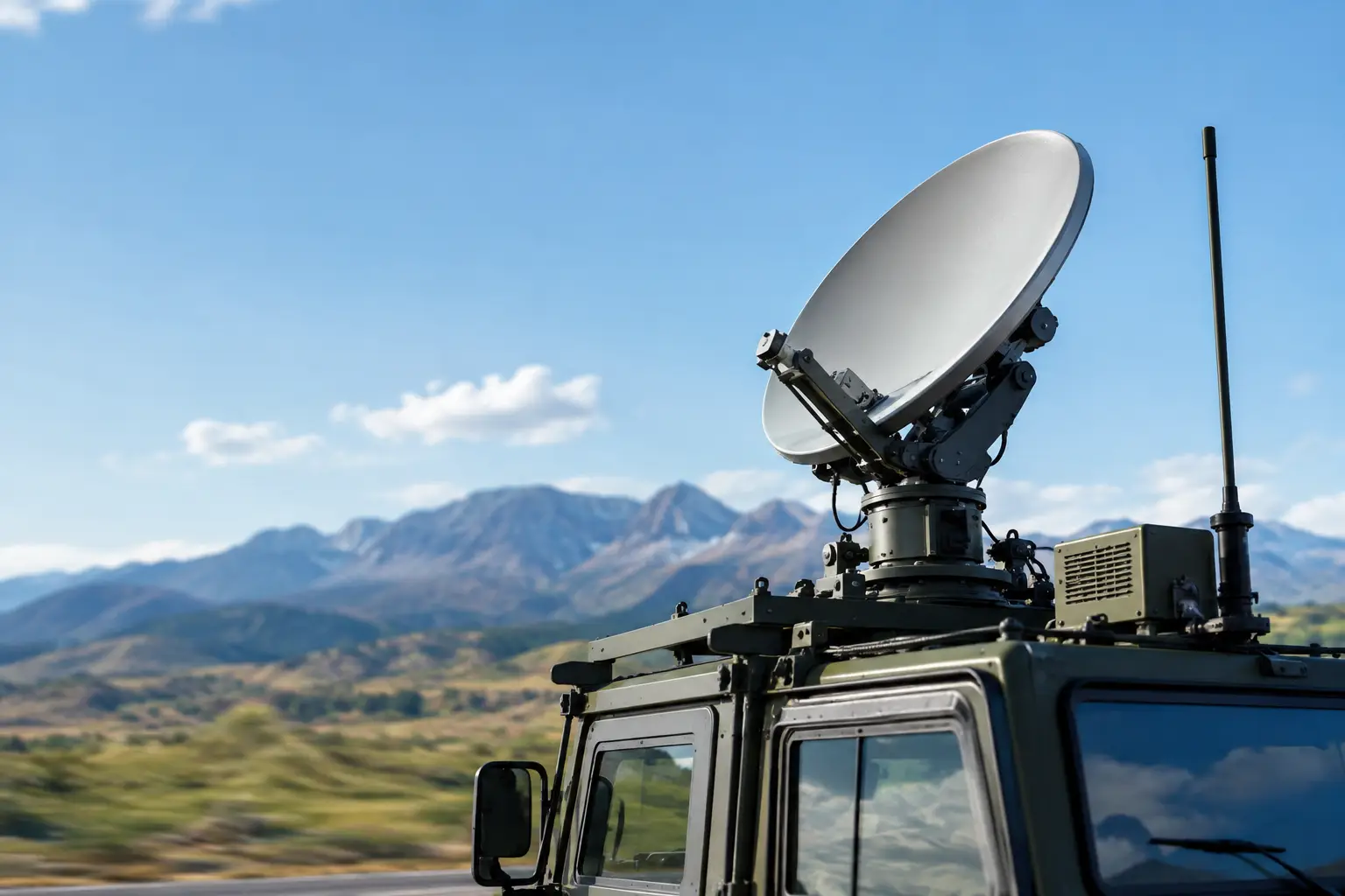
Antenna gain concentrates RF energy. High-gain antennas can extend a path or improve fade margin, provided both ends of the link maintain the required alignment. In fixed deployments, this may be achieved with careful installation and rigid mounting. In mobile environments, the problem is different: antenna pointing must compensate for pitch, roll, yaw, vibration, or changing vehicle direction.

This is where auto-aiming and stabilized antenna systems become part of the link budget conversation. Their value is not merely convenience. They help preserve the antenna gain assumed in the design. If a narrow-beam antenna is off target, its effective gain can fall quickly enough to consume the margin that kept the link reliable.

Polarization must also match. Cross-polarization loss can be significant, especially in systems where antennas rotate or where mounting constraints make consistent orientation difficult. Dual-polarized systems can support higher capacity, but they require disciplined design and installation to realize that benefit.

Feedline, Connector, and Equipment Losses

Losses between the radio and antenna are frequently underestimated. Coaxial cable loss increases with frequency and cable length. Connectors, lightning protection devices, waveguide transitions, splitters, and damaged terminations all add insertion loss.

At microwave and millimeter-wave frequencies, locating the radio close to the antenna can materially improve performance by reducing feedline loss. This is one reason integrated radio and antenna designs are common in high-capacity outdoor systems. The architecture reduces loss points and simplifies field troubleshooting, though it may change maintenance access and power planning requirements.

Free-Space Path Loss

Free-space path loss is the signal reduction caused by RF energy spreading as it travels through open space. It rises as distance increases and rises further at higher frequencies. A 20-mile path at one band is not directly comparable to a 20-mile path at another.

Free-space path loss is predictable, which makes it a useful foundation for a design. It is not, however, the complete path model. Terrain, water reflections, Fresnel-zone obstruction, atmospheric absorption, rain, and localized interference can materially change actual performance.

For links over water, the path may appear visually clear while multipath reflections create deep fading. For industrial sites, cranes, structures, stacked materials, and moving equipment may intermittently obstruct the path. For ground-to-air networks, range changes continuously and antenna tracking accuracy becomes a central performance variable.

Receiver Sensitivity and Required Throughput

Receiver sensitivity is the minimum signal level a receiver needs to decode a signal at a defined performance level. It is not one fixed number. Sensitivity changes with channel width, modulation and coding scheme, data rate, receiver noise figure, and acceptable error rate.

A link may remain connected at a low modulation level while losing the throughput required for video, telemetry, voice, SCADA traffic, or private cellular backhaul. The correct design target is therefore not simply connection status. It is the required capacity and availability at the operational edge of the network.

Higher-order modulation can deliver more data but needs a cleaner, stronger signal. Lower-order modulation can maintain service at weaker levels but reduces throughput. Adaptive modulation is valuable because it lets a system degrade gracefully, but it cannot replace sufficient fade margin when high availability is required.

Why Fade Margin Determines Real-World Reliability

Fade margin is the amount by which predicted received signal exceeds receiver sensitivity. It is the reserve that absorbs changes the static calculation cannot fully control.

The needed margin depends on the application. A temporary construction-site connection with noncritical office traffic may tolerate lower availability than a public safety command network, offshore crew welfare system, or backhaul path carrying multiple operational services. A short, fixed link in a dry environment needs different allowances than a long maritime link exposed to weather, motion, and reflected signal paths.

Engineers should account for likely degradations, including rain fade at higher frequencies, atmospheric loss, vegetation, Fresnel-zone encroachment, interference, antenna radome loss, and mechanical movement. For mobile or maritime systems, tracking error and platform motion should be treated as budget factors, not afterthoughts.

A generous fade margin does not mean selecting the largest antenna and highest-power radio in every case. Oversizing can raise cost, wind loading, power demand, spectrum coordination challenges, and deployment complexity. The objective is an engineered balance between availability, capacity, compliance, and lifecycle cost.

How to Build a Link Budget That Holds Up in the Field

Start with the service requirement: required throughput, latency expectations, availability target, traffic priority, frequency band, and operating environment. Then define the path in practical terms. Map distance, elevation, line of sight, Fresnel-zone clearance, likely obstructions, mounting locations, and the movement profile of any mobile endpoint.

Next, use verified equipment data. Include radio output at the intended modulation, actual antenna gain, cable and connector losses, and receiver sensitivity for the desired channel width and capacity. Vendor maximum values can be misleading when they apply only to a different channel configuration, regulatory domain, or modulation mode.

Model environmental and operational losses explicitly. A fixed tower-to-tower path may require a terrain and obstruction assessment. A stabilized microwave link should include the expected pointing accuracy under vessel or vehicle motion. A private 5G backhaul design should consider both the backhaul path and the access network demand that will ride over it.

Finally, validate the calculation after deployment. Measure received signal level, signal-to-noise ratio, modulation behavior, packet loss, throughput, and performance during adverse conditions. Field measurements reveal issues that desktop planning cannot always predict, such as intermittent interference, poor grounding, incorrect polarization, or reflections from nearby structures.

Link Budget Is a System Design Discipline

A link budget is most useful when it is treated as a living engineering record rather than a one-time spreadsheet. As path conditions, capacity needs, or equipment configurations change, the budget should be updated to show whether the original availability target still holds.

For demanding deployments, the strongest result comes from designing the radio, antenna, mounting system, tracking capability, path geometry, and service requirement as one system. That approach turns a calculated RF path into a communications link that can keep performing when the operating environment becomes less forgiving.